

Duplicates can occur regardless of how carefully you enter or import data. While you could detect and eliminate duplicates, you might wish to evaluate them instead. We’ll teach you how to use Google Sheets to spot duplicates.
You may have a list of client email addresses and phone numbers, product IDs and order numbers, or other data that should not contain duplicates. You may then check and repair the inaccurate data by detecting and marking duplicates in your spreadsheet.
While Microsoft Excel‘s conditional formatting makes it simple to spot duplicates, Google Sheets does not presently offer this feature. Using a custom formula in addition to conditional formatting, you may indicate duplicates in your sheet.
Sign in to Google Sheets and navigate to the spreadsheet you wish to work on. Choose the cells where you wish to look for duplicates. A column, row, or cell range can be used.

Select Format > Conditional Formatting from the menu. This brings up the Conditional Formatting sidebar, where you may create a rule to identify duplicate data.

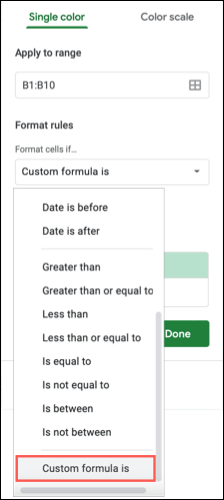
Select the Single Color tab at the top sidebar and confirm the cells beneath Apply to Range.

Open the Format Cells If a drop-down box, then click “Custom Formula Is” at the bottom of the list.
In the Value or Formula box that appears beneath the drop-down box, enter the following formula. In the formula, replace the letters and cell reference with those from your chosen cell range.
=COUNTIF(B:B,B1)>1
COUNTIF is the function, in this case, B: B is the range (column), B1 is the condition, and >1 is more than one.
You may also use the following formula for accurate cell references as the range.
=COUNTIF($B$1:$B$10,B1)>1
COUNTIF is the function here, the range is $B$1:$B$10, B1 is the condition, and >1 is more than one.
Select the sort of highlight you wish to use under Formatting Style. To select a color from the palette, click the Fill Color icon. If you wish, you may format the font in the cells with bold, italic, or a color.

When you’re finished applying the conditional formatting rule, click “Done.” The cells containing duplicate data should be formatted in the way you choose.

As you make changes to the duplicate data, the conditional formatting will vanish, leaving you with the remaining duplicates.
In Google Sheets, you may quickly update a rule, add a new one, or delete one. Select Format > Conditional Formatting to open the sidebar. You’ll see the rules you’ve established.

You may start rectifying incorrect data by detecting and marking duplicates in Google Sheets. If you’re looking for more methods to utilize conditional formatting in Google Sheets, have a look at how to apply a color scale based on value or how to highlight blanks or cells with mistakes.

ManilaShaker is a tech media producing insightful and helpful content for our local and growing international audience. Our goal is to create a premier Philippine digital consumer electronics resource that provides the most objective reviews and comparisons globally.


