

You may quickly and easily present data using graphs and charts. However, what if you want to concentrate on a specific area of your chart? You may highlight particular data in an Excel chart by using a filter.
Using a convenient button, Microsoft Excel for Windows allows you to rapidly filter your chart data. Although this feature is not yet available in Excel for Mac, you may still filter the data to refresh the chart. Let’s examine both!
Filter a Chart in Excel on Windows
The data filter in Excel is definitely available on the Home tab. On Windows, though, Microsoft makes the process of filtering a chart a little bit easier.
When you select the chart, buttons will appear to the right of it. Select Chart Filters from the menu (funnel icon).
 Select the Values tab at the top of the filter box when it appears. After that, you can enlarge and filter by Series, Category, or both. Simply select the options on the chart that you want to see, then click “Apply.”
 Be aware that several chart kinds, like Pareto, Histogram, and Waterfall charts, do not include the Chart Filters option. By using a filter on the data rather than the chart, you can still filter the latter. The procedures for filtering a chart in Excel on a Mac are the same as those in Excel on a Windows computer.
Remove a Filter
When you finish using the Chart Filters, click that button once more to open the filter box. Check the boxes for Select All in Series or Categories, depending on the filter you used. Then, click “Apply.”
 Your chart should then be back to its original view.
Filter a Chart in Excel on Mac
You must use the data filter on the Home tab because an Excel for Mac chart doesn’t have a Chart Filters button next to it.
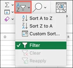
Choose your chart’s data, not the graphic itself. Select “Filter” from the drop-down menu at the top of the Sort & Filter ribbon by clicking the Home tab.
 Click the arrow at the top of the column for the chart data you want to filter. Use the Filter section of the pop-up box to filter by color, condition, or value.
 When you finish, click “Apply Filter” or check the box for Auto Apply to see your chart update immediately.
Remove a Filter
Remove the filter to restore your chart to its default view. When a pop-up box appears, click the filter button at the top of the column you want to clear.
![]()
You can also choose to disable the data filter. Going back to the Home tab, selecting “Filter” on the Sort & Filter ribbon, and then deselecting it
Charts can benefit from filters as well as data sets. Thus, keep this advice in mind the next time you wish to highlight data in an Excel pie, column, or bar chart.

ManilaShaker is a tech media producing insightful and helpful content for our local and growing international audience. Our goal is to create a premier Philippine digital consumer electronics resource that provides the most objective reviews and comparisons globally.


